Analytic Methods to Examine Changes Across Years Using HINTS 2003 & 2005 Data
Division of Cancer Control and Population Sciences
National Cancer Institute
U.S. Department of Health and Human Services
Lou Rizzo, Ph.D.1
Richard P. Moser, Ph.D.2
William Waldron, B.S.3
Zhuoqiao Wang, M.S.3
William W. Davis, Ph.D.2
1Westat Inc.;
2Division of Cancer Control and Population Sciences, National Cancer Institute;
3Information Management Services, Inc.
1. Introduction
2. Three Types of Anaylses Using Multiple Biennial HINTS Surveys
3. Goal 1—Estimating Changes Without Controlling for Other Factors
4. Combining the Data Files
5. Goal 2—Estimating Changes Controlling for Other Factors
6. Goal 3— Estimating Averages by Combining 2003 and 2005 Data
7. Other Analyses
References
Appendix A. SAS/SUDAAN Code for Carrying Out the Calculations
Appendix B. STATA Code for carrying out the Calcuations
Appendix C. Computing Degrees of Freedom
Cancer Information and Resources
1. INTRODUCTION
The Health Information National Trends Survey (HINTS) is a national, biennial survey designed to collect nationally representative data on the American public's need for, access to, and use of cancer-related information. The primary task of HINTS is to monitor changes in the rapidly evolving field of health communication. This survey is sponsored and directed by the National Cancer Institute's Division of Cancer Control and Population Sciences. The baseline year is 2003, and data from the first follow-up sample in 2005 are also available (see https://hints.cancer.gov). A second follow-up sample (for 2007) is currently being implemented.
Each biennial sample is drawn using a random-digitdial (RDD) sample design to produce a representative sample of telephone households in the country. Exchanges with high percentages of Blacks and Hispanics were oversampled in 2003, in order to provide a larger yield of these important subgroups. In a second stage of selection, one adult was randomly selected among all adults living in the sampled household. This adult was recruited to complete the main survey instrument by telephone interview4.
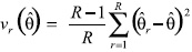
Weights are assigned to account for all of the stages of selection (from the RDD sampling frame and within the household), and for attrition from noncontacts, screener nonresponse, and interview nonresponse. These weights are designed to provide approximately unbiased estimators of population totals using a modified Horvitz-Thompson estimator (see for example Cochran 1977, Section 9A.7)5. Replicate weights are also provided to allow for consistent variance estimation. The replicate weights for all of the biennial HINTS surveys are based on the jackknife replication method, with R = 50 replicate weights for each survey year. The replicate weights are formed by deleting a carefully selected portion of the original sample (roughly 1/50 of the original sample), and reweighting the remaining sample as if the complement set was the full sample. Estimates are computed using each set of replicate weights, generating a set of parallel replicate estimates to the estimate of interest. The sum of squares of the deviations between the replicate estimates and the ‘full-sample’ estimate, with appropriate adjustment, provides consistent estimators of the variance. For example, suppose
 is an estimator (a percentage within a subgroup, for example) using the ‘fullsample’ weights. We generate replicate estimators
r in parallel, doing the calculation in the same way, but using each set of replicate weights in place of the original full-sample weights. The jackknife variance estimator of
is
is an estimator (a percentage within a subgroup, for example) using the ‘fullsample’ weights. We generate replicate estimators
r in parallel, doing the calculation in the same way, but using each set of replicate weights in place of the original full-sample weights. The jackknife variance estimator of
is
Final methodology reports are available for both HINTS 2003 and HINTS 2005 and are accessible online at no cost on https://hints.cancer.gov. These reports provide details of the sampling and weighting for the respective surveys. This methodology paper is closely based on a similar methodology paper (Lee, et al. 2007) for the California Health Information Survey (CHIS).
4In HINTS 2005, a small number of persons completed interviews via the Internet, as part of an experimental study nested within the main HINTS survey.
5Nonresponse is viewed as a further ‘pseudo’ stage of sampling, in which it is assumed that respondents are a simple random sample from all sampled persons within carefully defined response cells (the ‘pseudo-randomization paradigm’: see for example Oh and Scheuren 1983).
Back to top
2. THREE TYPES OF ANALYSES USING MULTIPLE BIENNIAL HINTS SURVEYS
Throughout this document, we will provide examples of HINTS analyses, using as our primary outcome for each example an estimate from HINTS of the percentage of respondents who ever looked for cancer information using the Internet6. Table 2 below presents the estimates from HINTS 2003 and HINTS 2005 for the overall population and for sociodemographic subgroups of general interest, as well as standard errors (the square roots of the jackknife variance estimates).
Research based on a series of cross-sectional surveys often emphasizes the results of the new survey but also includes testing for changes between survey iterations, i.e., examining trends in responses to a given survey item over time. This document focuses on three general goals and provides SAS/SUDAAN and STATA syntax examples for each when making inferences from multiple cross-sectional surveys:
Table 2 Estimates of percentages of adults who have ever looked for cancer information online.
SUBGROUP |
2003 |
2005 |
| Weighted % |
Standard Error |
Weighted % |
Standard Error |
| ALL |
19.7% |
0.6% |
28.3% |
0.7% |
| |
Age
18–34 |
23.5% |
1.3% |
32.6% |
1.5% |
| 35–49 |
23.3% |
1.2% |
32.5% |
1.6% |
| 50–64 |
20.6% |
1.2% |
30.0% |
1.4% |
| 65+ |
4.2% |
0.5% |
9.6% |
0.8% |
| |
Education Level
Less than high school |
6.5% |
1.4% |
6.4% |
1.1% |
| High school graduate |
12.0% |
0.9% |
19.9% |
1.6% |
| Some college |
23.9% |
1.3% |
34.7% |
1.9% |
| College graduate or more |
36.0% |
1.3% |
46.5% |
1.6% |
| |
Race
Non-Hispanic White |
23.1% |
0.8% |
33.3% |
1.1% |
| Non-Hispanic Black |
13.6% |
1.7% |
23.3% |
3.4% |
| Hispanic |
7.2% |
1.0% |
11.2% |
2.0% |
| Non-Hispanic Other |
22.1% |
2.4% |
28.2% |
3.7% |
| |
Gender
Male |
16.7% |
0.8% |
25.3% |
1.4% |
| Female |
22.4% |
0.9% |
31.0% |
0.9% |
| |
Annual Income
Less than $25,000 |
10.1% |
0.9% |
18.0% |
1.5% |
| $25,000 to $49,999 |
16.6% |
1.2% |
25.6% |
1.9% |
| $50,000 to $74,999 |
27.3% |
1.6% |
30.4% |
2.0% |
| $75,000 or more |
36.3% |
1.8% |
44.6% |
2.1% |
- Goal 1: Estimating a change in a characteristic such as a mean or a percentage and testing the statistical significance of the change (across and within subgroups):
- Example 1: Has the percentage of persons who have ever looked for cancer information online changed between 2003 and 2005? What is the estimate of the change?
- Example 2: Has the percentage of Black persons who have ever looked for cancer information online changed between 2003 and 2005? What is the estimate of the change?
- Goal 2: Estimating a change in a characteristic while controlling for covariates (across and within subgroups):
- Example 1: Has the percentage of persons who have ever looked for cancer information online changed in the last two years, after controlling for age, education level, and gender?
- Example 2: Has the percentage of college graduates who have ever looked for cancer information online changed in the last two years, after controlling for age and gender?
- Goal 3: Estimating the average using data from multiple survey years assuming that the mean has not changed between those years:
- What is the average percentage of persons who have ever looked for cancer information Online over the period 2003–2005?
Note that Goals 1 and 2 are relevant to test for differences or change in responses to survey items that are identical (or comparable) across years, while Goal 3 would be used to combine across years to obtain one larger sample size.
6The exact derivation of the example percentage from the HINTS questionnaire items is given in Appendix A.
Back to top
3. GOAL 1–ESTIMATING CHANGES WITHOUT CONTROLLING FOR OTHER FACTORS
It is easy to produce an estimate of change in characteristics between 2003 and 2005 and its corresponding variance estimate, because HINTS samples are drawn independently. Here we will label HINTS 2003 "year 1" and HINTS 2005 "year 2," and consider estimating a characteristic θ (e.g., a mean, percentage, regression coefficient, population standard deviation) in year s. We label the true value in year s as θs, the estimated value as
s, and the estimated variance (the square of the standard error) as ν(s). The true change between years is Δ=θ2-θ1, with consistent estimator
 =2-1
=2-1
Because the samples are independent, the variance is the sum of the two variances, and a consistent variance estimator is
ν()=ν(1)+ν(2)
Table 3-1 provides a summary of this information.
Table 3-1 Summary of Estimating Changes Using Two Independent Surveys.
| Year |
True Value |
Estimated Value |
Variance of Estimate |
| 1 |
θ1 |
1 |
ν(1) |
| 2 |
θ2 |
2 |
ν(2) |
| Change |
Δ=θ2-θ1 |
=2-1 |
ν()=ν(1)-ν(2) |
A hypothesis test for the null hypothesis of no change (θ1 = θ2) can be tested against a one-sided (θ1 < θ2) or two-sided (θ1 ≠ θ2) alternative. The one-sided alternative may be more appropriate when any change that occurs is expected to be positive change (such as in the degree of Internet usage). The test statistic is

For national estimates (in contrast to subgroups) this can be referred to a t-distribution, using either the one-sided tα,df or the two-sided tα/2,df. Finding the correct number of degrees of freedom is not a trivial task. Appendix C provides a method (Welch's method) for approximating the number of degrees of freedom, and shows why the t distribution on 49 degrees of freedom will be the most conservative (i.e., giving the widest confidence intervals), thereby reducing the likelihood of committing a Type I error. Using Welch's method, the number of degrees of freedom will be something between 49 and 98. It should be noted that all of these t-distributions are close to each other, and close to the standard normal distribution (i.e., the corresponding percentiles are nearly equal).
For most applications for HINTS, the Welch approximation assuming 49 degrees of freedom for each year will be reasonable. The degrees of freedom for the chi-square distribution can be no larger than the set of independent nonzero squares that underlies the variance estimator. Suppose for example that a particular estimate is restricted to a limited subgroup of the sample, so that many of the replicate squared deviations are negligibly close to zero (see the equation for vr() at the end of Section 1). In this case, a smaller number of degrees of freedom should be used7. SAS/SUDAAN does allow the user to specify degrees of freedom if the user wishes to overrule the software's choice. It should be noted that without manual specification the SAS/SUDAAN program uses as degrees of freedom the total number of replicates, and the STATA software uses as degrees of freedom: the total number of replicates minus 1 respectively. STATA doesn’t appear to allow for any re-specification of degrees of freedom. These degrees of freedom are ‘liberal’ (just beyond the high end of the ‘acceptable’ range as per the Welch method).
Table 3-2 on the next page presents one-sided and two-sided p-values for the null hypothesis of no change between 2003 and 2005 in percentages of adults who had ever looked for cancer information online, both for all adults and for a number of socioeconomic subgroups. Table 3-3 presents corresponding confidence intervals. The Table 3-2 and 3-3 values were computed separate from the two HINTS data sets (using STATA and SAS/SUDAAN to do these separate-year computations), with differences, standard errors, p-values, and confidence intervals computed in Excel, using a t-distribution on 98 degrees of freedom. If the p-value percentage in the table is more than 5% (for example), one would not reject the hypothesis at the 5% significance level. The table shows that for all but four groups (less than high school, Hispanic, non-Hispanic other, and $50,000–$74,999) we would reject the two-sided test of no change at the 5% significance level. Note that the results for ‘all’ and for ‘non-Hispanic Black’ can be used to test the hypotheses for Goal 1: Examples 1 and 2 respectively.
The rows of the table allow the test of 19 hypotheses. If we wish to control the Type I error to 5% over all these hypotheses, we should use a significance level smaller than 5% for each individual test. The most conservative approach is the Bonferroni approach, in which the cutoff p-value is 5% / 19, or 0.26% as a cutoff. Many of the p-values in Table 3-2 pass this most conservative test. These can be confidently viewed as significant results. There are many other multiple comparisons tests that are less conservative than the Bonferroni approach; these are available in the current versions of both SAS and STATA for example.
Table 3-2 Estimates of differences of percentages of adults who have ever looked for cancer information online,
between 2003 and 2005.
| SUBGROUP |
2003 Weighted Estimate
1 |
Standard Error
 |
2005 Weighted Estimate
2 |
Standard Error
 |
Estimate of 2003 to 2005 Change
 |
Standard Error
 |
Two-sided p-value of Test of No Change8 |
One-sided p-value of Test of No Change8 |
| ALL |
19.7% |
0.6% |
28.3% |
0.7% |
8.6% |
0.9% |
0.0000% |
0.0000% |
| |
Age
18–34 |
23.5% |
1.3% |
32.6% |
1.5% |
9.1% |
2.0% |
0.0013% |
0.0007% |
| 35–49 |
23.3% |
1.2% |
32.5% |
1.6% |
9.3% |
2.0% |
0.0014% |
0.0007% |
| 50–64 |
20.6% |
1.2% |
30.0% |
1.4% |
9.4% |
1.8% |
0.0001% |
0.0001% |
| 65+ |
4.2% |
0.5% |
9.6% |
0.8% |
5.4% |
0.9% |
0.0000% |
0.0000% |
| |
Education Level
Less than high school |
6.5% |
1.4% |
6.4% |
1.1% |
-0.1% |
1.7% |
96.77% |
48.39% |
| High school graduate |
12.0% |
0.9% |
19.9% |
1.6% |
8.0% |
1.8% |
0.0033% |
0.0016% |
| Some college |
23.9% |
1.3% |
34.7% |
1.9% |
10.7% |
2.4% |
0.0014% |
0.0007% |
| College graduate or more |
36.0% |
1.3% |
46.5% |
1.6% |
10.5% |
2.1% |
0.0002% |
0.0001% |
| |
Race
Non-Hispanic White |
23.1% |
0.8% |
33.3% |
1.1% |
10.1% |
1.3% |
0.0000% |
0.0000% |
| Non-Hispanic Black |
13.6% |
1.7% |
23.3% |
3.4% |
9.6% |
3.8% |
1.22% |
0.61% |
| Hispanic |
7.2% |
1.0% |
11.2% |
2.0% |
4.1% |
2.2% |
7.36% |
3.68% |
| Non-Hispanic Other |
22.1% |
2.4% |
28.2% |
3.7% |
6.1% |
4.4% |
16.58% |
8.29% |
| |
Gender
Male |
16.7% |
0.8% |
25.3% |
1.4% |
8.6% |
1.7% |
0.0001% |
0.0001% |
| Female |
22.4% |
0.9% |
31.0% |
0.9% |
8.6% |
1.2% |
0.0000% |
0.0000% |
| |
Annual Income
Less than $25,000 |
10.1% |
0.9% |
18.0% |
1.5% |
7.9% |
1.8% |
0.0021% |
0.0011% |
| $25,000 to $49,999 |
16.6% |
1.2% |
25.6% |
1.9% |
9.0% |
2.2% |
0.0101% |
0.0051% |
| $50,000 to $74,999 |
27.3% |
1.6% |
30.4% |
2.0% |
3.1% |
2.5% |
22.85% |
11.42% |
| $75,000 or more |
36.3% |
1.8% |
44.6% |
2.1% |
8.3% |
2.8% |
0.34% |
0.17% |
One can compute one-sided or two-sided confidence intervals of the difference using similar considerations. The two-sided confidence interval will be
![delta hat plus or minus t sub [{alpha divided by two} comma degrees of freedom] times the square root of the estimated variance of theta hat; square root of the estimated variance of delta hat](/_images/scientific_equations-6.jpg)
tα/2,df is the two-sided cutoff point using a t distribution on df degrees of freedom. Checking whether this confidence interval contains zero is equivalent to the two-sided test of the null hypothesis of no change using the corresponding t-distribution. Table 3-3 presents two-sided confidence intervals using the t-distribution for the change in percentage of adults who have ever looked for cancer information online (note that the first two columns of Table 3-3 give the same difference estimates as Table 3-2: they are included here as well as they are the center values of the confidence intervals from the two-sided test). Again, the table shows that for all but four groups (less than high school, Hispanic, non-Hispanic other, and $50,000–$74,999) we would reject the two-sided test of no change at the 5% significance level (since the confidence intervals include zero for these four groups).
Table 3-3 Confidence intervals for differences in percentages of adults who have ever looked for cancer information online, between 2003 and 2005.
| SUBGROUP |
Estimate of 2003 to 2005 Change
|
Standard Error
|
Lower Bound 95% C.I. |
Upper Bound 95% C.I. |
| ALL |
8.6% |
0.9% |
6.8% |
10.4% |
| |
Age
18–34 |
9.1% |
2.0% |
5.2% |
13.1% |
| 35–49 |
9.3% |
2.0% |
5.3% |
13.3% |
| 50–64 |
9.4% |
1.8% |
5.8% |
13.1% |
| 65+ |
5.4% |
0.9% |
3.6% |
7.2% |
| |
Education Level
Less than high school |
-0.1% |
1.7% |
-3.5% |
3.4% |
| High school graduate |
8.0% |
1.8% |
4.3% |
11.6% |
| Some college |
10.7% |
2.4% |
6.1% |
15.4% |
| College graduate or more |
10.5% |
2.1% |
6.4% |
14.5% |
| |
Race
Non-Hispanic White |
10.1% |
1.3% |
7.6% |
12.7% |
| Non-Hispanic Black |
9.6% |
3.8% |
2.1% |
17.1% |
| Hispanic |
4.1% |
2.2% |
-0.4% |
8.5% |
| Non-Hispanic Other |
6.1% |
4.4% |
-2.6% |
14.8% |
| |
Gender
Male |
8.6% |
1.7% |
5.3% |
11.8% |
| Female |
8.6% |
1.2% |
6.1% |
11.1% |
| |
Annual Income
Less than $25,000 |
7.9% |
1.8% |
4.4% |
11.5% |
| $25,000 to $49,999 |
9.0% |
2.2% |
4.6% |
13.3% |
| $50,000 to $74,999 |
3.1% |
2.5% |
-2.0% |
8.1% |
| $75,000 or more |
8.3% |
2.8% |
2.8% |
13.7% |
7A procedure recommended here is to consider as ‘negligible’ any replicate square in the set of replicate squares that is less than 1% of the median square, which will eliminate spurious ‘essentially nonzero’ squares.The software packages do not currently do this or anything similar to it, so the interested user will need to do this in a ‘manual’ way.
8Note that these are percentages: .0021% is .000021, 5.2% is .052.This allows for greater clarity (more significant digits).
Back to top
4. COMBINING THE DATA FILES
For Goal 1, it is only necessary to have the separate 2003 and 2005 data sets, compute the estimates and standard errors, compute differences by subtracting the two sets of estimates, and compute standard errors for those differences by adding the two variances. For Goals 2 and 3 and any more sophisticated analyses, combining the data files will be necessary. It turns out that if the data files are combined properly, the analyses of Goal 1 can also be easily reproduced using the combined data set.
The main purpose of Goal 3 is to allow an augmented sample size: both years can be combined, virtually doubling the sample size. This will considerably improve precision for those characteristics which do not change much between the years.
To create the combined data file, one can concatenate the 2003 and 2005 public use files so that the number of respondents in the combined data file is the sum of the respondents from the two individual data files. Two main tasks are required to combine the data files. First, variables used in the analyses should have the same name and values or categories in both data files. Section A of the Appendix describes how variables are redefined for the tasks in this document. Second, create a set of new statistical weights as shown in Table 4. There will be 101 weights in the combined data file: 1 final weight and 100 replicate weights. We label them NFWGT and NFWGT1–NFWGT100. The final weight (NFWGT) in the combined file is created by using the final weight (FWGT) from the respective surveys.
For the first 50 replicate weights (NFWGT1, …, NFWGT50), we use replicate weights FWGT1, … ,FWGT50 from the sample persons from the HINTS 2003 survey, and we use the final weight FWGT (for all 50 replicates) for sample persons from the HINTS 2005 survey. Replicate weights equal to the final weight essentially result in zero sums of squares contributed to the variance estimator from those replicates. For the first 50 replicate weights, only the HINTS 2003 survey contributes variance. For the remaining 50 replicate weights (NFWGT51, …, NFWGT100), we use replicate weights FWGT1, …, FWGT50 from the sample persons from the HINTS 2005 survey, and we use the final weight FWGT (for all 50 replicates) for sample persons from the HINTS 2003 survey. For replicate weights 51 through 100, only the HINTS 2005 survey contributes variance. When the sums of squares for all 100 replicates are put together, the result is a sum of HINTS 2003 and HINTS 2005 variance, as desired (as the surveys are in fact independent).
It is also necessary to define a YEAR field equal to 2003 (or 1) for HINTS 2003 sample members, and equal to 2005 (or 2) for HINTS 2005 sample members. The Goal 1
=
2 -
1, with corresponding standard errors, test statistics, and confidence intervals, can be easily (and correctly) estimated from this combined data set using a contrast with the YEAR field (+1 for HINTS 2005 records and -1 for HINTS 2003 records). Appendix A provides SAS syntax for computing the new replicate weights9 and SUDAAN syntax for calculating the estimate of the difference10. Appendix B provides corresponding STATA code11.
Table 4 Construction of statistical weights for the combined data file.
| |
Final Sample Weight |
Replicate Weights 1-50 |
Replicate Weights 51-100 |
| Hints 2003 |
2003 Final Weight (FWGT) |
2003 Replicate Weights (FWGT1-FWGT50) |
2003 Final Weight (FWGT) |
| Hints 2005 |
2005 Final Weight (FWGT) |
2005 Final Weight (FWGT) |
2005 Replicate Weights (FWGT1-FWGT50) |
| Combined Data |
Final Weight (NFWGT) |
Final Replicate Weights (NFWGT1-NFWGT50) |
Final Replicate Weights (NFWGT51-NFWGT100) |
9Under the title "Adjust replicate weights for the combined dataset".
10Under the title "Test for differences across years using combined dataset."
11Under the titles "Create the replicate weights for the combined data" and "Test for differences across years using combined data…".
Back to top
5. GOAL 2—ESTIMATING CHANGES CONTROLLING FOR OTHER FACTORS
The change estimates presented in Section 3 are marginal changes: they are composites of changes in internet usage within specified subgroups, and changes in the percentages of subgroups. For example, suppose there is a change in Internet usage, but it is entirely because one group which had a higher Internet usage is now a larger percentage of the population (all groups within themselves had no change in Internet usage). In general, analysts want to be able to distinguish these compositional changes from actual trends in the characteristic of interest.
In this section, we explore how to conduct analyses that search for ‘true’ non compositional changes in HINTS responses between 2003 and 2005. For example, Table 5-1 presents results from checking for 2003 to 2005 differences using logistic regression (with the binary dependent variable equal to 1 if ever Internet searched, and 0 otherwise). The beta coefficients represent effects on a log-odds12 scale: the estimated odds ratios are also given (the transformed beta coefficients). Age, education level, and gender are also main effects in this model, so the year change coefficient can be interpreted as a year-to-year change adjusting for changes in composition by age group, education level, and gender between the two years. The odds ratio for the 2005 to 2003 difference is 1.66: holding constant these other factors, the odds are 66% higher of ever having used the Internet to search for cancer information in 2005 as compared to 2003 (with a 95% confidence interval ranging from 48% to 87% higher). Since the 95% confidence interval for the odds ratio does not include 1, we would reject the hypothesis of no change for Goal 2 example 1. The table shows higher odds ratios for the younger age categories compared to the oldest category (65+) and lower odds ratios for the lower education groups compared to the highest education level group (‘college graduate or more’). The SAS/SUDAAN and STATA code for carrying out this calculation is given in Appendices A and B respectively.
Table 5-1 Changes in percentages of adults who have ever looked for cancer information online between 2003 and 2005 controlling for age, education level, and gender.
| SUBGROUP |
Beta Coefficient |
Standard Error Beta Coefficient |
Odds Ratio |
Lower Bound 95% CI Odds Ratio |
Upper Bound 95% CI Odds Ratio |
| INTERCEPT |
-1.74 |
0.11 |
0.17 |
0.14 |
0.22 |
| |
SURVEY YEAR
2003 |
0.00 |
0.00 |
1.00 |
1.00 |
1.00 |
| 2005 |
0.51 |
0.06 |
1.66 |
1.48 |
1.87 |
| |
AGE
18-34 |
1.57 |
0.10 |
4.78 |
3.93 |
5.83 |
| 35-49 |
1.45 |
0.09 |
4.27 |
3.57 |
5.13 |
| 50-64 |
1.32 |
0.10 |
3.75 |
3.06 |
4.60 |
| 65+ |
0.00 |
0.00 |
1.00 |
1.00 |
1.00 |
| |
EDUCATION LEVEL
Less than high school |
-2.24 |
0.16 |
0.11 |
0.08 |
0.15 |
| High school graduate |
-1.31 |
0.09 |
0.27 |
0.23 |
0.32 |
| Some college |
-0.59 |
0.08 |
0.55 |
0.47 |
0.64 |
| College graduate or more |
0.00 |
0.00 |
1.00 |
1.00 |
1.00 |
| |
GENDER
Male |
-0.36 |
0.07 |
0.70 |
0.60 |
0.81 |
| Female |
0.00 |
0.00 |
1.00 |
1.00 |
1.00 |
To summarize, the model underlying Table 5-1 imposes a structure that year-to-year differences only affect the intercept, and do not also show differences in the slopes for the other covariates. An interaction model can be used to test whether this assumption about the structure is correct. For example, there could have been more gain in ever having looked for cancer information online in the higher education groups than the lower education groups between 2003 and 2005.
Table 5-2 presents the results of a model in which education level is interacted with year. The ‘Education Level 2003’ parameters represent differences between each education level and the baseline education level (‘college graduate or more’) for the baseline year 2003. These would be the estimates for the main effects for education level in a traditionally structured table (see for example Korn and Graubard [1999], Table 8.4.4) which puts main effects first. The ‘Education Level 2005 vs. 2003’ estimates are the differences in education level parameter estimates between 2003 and 2005: the interaction between year (2005 to 2003) and education level. Note that the confidence intervals for the odds ratio for the three interaction terms contain 1, which indicates that there is not a strong interaction between education and survey year in this case. More formal tests of the hypothesis of no interaction between education and survey year, such as the Wald test, are available using both SAS/SUDAAN and STATA.
If the ‘Education Level 2003’ beta coefficients estimates and the ‘Education Level 2005 to 2003’ beta coefficient estimates are added together, the resultant summations for each education level are estimates for that education level (as against the baseline education level) for the year 2005.
Table 5-2 Changes in percentages of adults who have ever looked for cancer information online between 2003 and 2005 controlling for age, education level, and gender, with a year vs. education level interaction.
| SUBGROUP |
Beta Coefficient |
Standard Error Beta Coefficient |
Odds Ratio |
Lower Bound 95% CI Odds Ratio |
Upper Bound 95% CI Odds Ratio |
| INTERCEPT |
-1.73 |
0.10 |
0.18 |
0.15 |
0.22 |
| |
SURVEY YEAR
2003 |
0.00 |
0.00 |
1.00 |
1.00 |
1.00 |
| 2005 |
0.47 |
0.09 |
1.60 |
1.34 |
1.91 |
| |
AGE
18-34 |
1.57 |
0.10 |
4.80 |
3.94 |
5.84 |
| 35-49 |
1.46 |
0.09 |
4.29 |
3.58 |
5.14 |
| 50-64 |
1.32 |
0.10 |
3.75 |
3.06 |
4.60 |
| 65+ |
0.00 |
0.00 |
1.00 |
1.00 |
1.00 |
| |
GENDER
Male |
-0.36 |
0.07 |
0.70 |
0.60 |
0.81 |
| Female |
0.00 |
0.00 |
1.00 |
1.00 |
1.00 |
| |
EDUCATION LEVEL 2003
Less than high school |
-1.97 |
0.25 |
0.14 |
0.09 |
0.23 |
| High school graduate |
-1.40 |
0.11 |
0.25 |
0.20 |
0.31 |
| Some college |
-0.64 |
0.09 |
0.53 |
0.44 |
0.64 |
| College graduate or more |
0.00 |
0.00 |
1.00 |
1.00 |
1.00 |
| |
EDUCATION LEVEL 2005 VS 2003
Less than high school |
-0.52 |
0.32 |
0.60 |
0.32 |
1.13 |
| High school graduate |
0.16 |
0.17 |
1.17 |
0.83 |
1.65 |
| Some college |
0.08 |
0.15 |
1.09 |
0.81 |
1.46 |
| College graduate or more |
0.00 |
0.00 |
1.00 |
1.00 |
1.00 |
For example, the odds ratio of 1.60 for 2005 vs. 2003 should be read in this case as a ratio of odds for 2005 college graduates to 2003 college graduates (college graduates are the referent category). The corresponding 2005 to 2003 ratio for ‘some college’ is 1.6 * (1.09) = 1.75, for ‘less than high school’ is 1.6 * (0.6) = 0.96. Table 5-2 allows one to ‘answer’ the Example 2 question under Goal 2 in Section 2. One can also extend the interactions between education level and the other predictors by doing separate analyses using education level as a subgroup. The slope coefficients are individual to that education level subgroup. Tables 5-3-1 through 5-3-4 present these results.
Table 5-3-1 Changes in percentages of adults who have ever looked for cancer information online between 2003 and 2005 controlling for age and gender, subsetted to the education level subgroup ‘less than high school’.
| SUBGROUP |
Beta Coefficient |
Standard Error Beta Coefficient |
Odds Ratio |
Lower Bound 95% CI Odds Ratio |
Upper Bound 95% CI Odds Ratio |
| INTERCEPT |
-4.41 |
0.44 |
0.01 |
0.01 |
0.03 |
| |
SURVEY YEAR
2003 |
0.00 |
0.00 |
1.00 |
1.00 |
1.00 |
| 2005 |
-0.07 |
0.30 |
0.93 |
0.51 |
1.68 |
| |
AGE
18-34 |
2.53 |
0.48 |
12.61 |
4.91 |
32.41 |
| 35-49 |
1.76 |
0.50 |
5.84 |
2.17 |
15.72 |
| 50-64 |
1.33 |
0.57 |
3.78 |
1.22 |
11.77 |
| 65+ |
0.00 |
0.00 |
1.00 |
1.00 |
1.00 |
| |
GENDER
Male |
-0.08 |
0.33 |
0.92 |
0.48 |
1.76 |
| Female |
0.00 |
0.00 |
1.00 |
1.00 |
1.00 |
Table 5-3-2 Changes in percentages of adults who have ever looked for cancer information online between 2003 and 2005 controlling for age and gender, subsetted to the education level subgroup ‘high school graduate’.
| SUBGROUP |
Beta Coefficient |
Standard Error Beta Coefficient |
Odds Ratio |
Lower Bound 95% CI Odds Ratio |
Upper Bound 95% CI Odds Ratio |
| INTERCEPT |
-3.43 |
0.24 |
0.03 |
0.02 |
0.05 |
| |
SURVEY YEAR
2003 |
0.00 |
0.00 |
1.00 |
1.00 |
1.00 |
| 2005 |
0.64 |
0.14 |
1.90 |
1.45 |
2.49 |
| |
AGE
18-34 |
1.97 |
0.23 |
7.15 |
4.55 |
11.25 |
| 35-49 |
1.91 |
0.22 |
6.76 |
4.33 |
10.55 |
| 50-64 |
1.62 |
0.25 |
5.03 |
3.04 |
8.34 |
| 65+ |
0.00 |
0.00 |
1.00 |
1.00 |
1.00 |
| |
GENDER
Male |
0.55 |
0.18 |
0.58 |
0.40 |
0.82 |
| Female |
0.00 |
0.00 |
1.00 |
1.00 |
1.00 |
Table 5-3-3 Changes in percentages of adults who have ever looked for cancer information online between 2003 and 2005 controlling for age and gender, subsetted to the education level subgroup ‘some college’.
| SUBGROUP |
Beta Coefficient |
Standard Error Beta Coefficient |
Odds Ratio |
Lower Bound 95% CI Odds Ratio |
Upper Bound 95% CI Odds Ratio |
| INTERCEPT |
-2.28 |
0.16 |
0.10 |
0.07 |
0.14 |
| |
SURVEY YEAR
2003 |
0.00 |
0.00 |
1.00 |
1.00 |
1.00 |
| 2005 |
0.56 |
0.12 |
1.74 |
1.38 |
2.20 |
| |
AGE
18-34 |
1.49 |
0.17 |
4.44 |
3.15 |
6.26 |
| 35-49 |
1.46 |
0.17 |
4.33 |
3.09 |
6.06 |
| 50-64 |
1.31 |
0.18 |
3.72 |
2.61 |
5.29 |
| 65+ |
0.00 |
0.00 |
1.00 |
1.00 |
1.00 |
| |
GENDER
Male |
-0.50 |
0.13 |
0.61 |
0.47 |
0.78 |
| Female |
0.00 |
0.00 |
1.00 |
1.00 |
1.00 |
Table 5-3-4 Changes in percentages of adults who have ever looked for cancer information online between 2003 and 2005 controlling for age and gender, subsetted to the education level subgroup ‘college graduate or more’.
| SUBGROUP |
Beta Coefficient |
Standard Error Beta Coefficient |
Odds Ratio |
Lower Bound 95% CI Odds Ratio |
Upper Bound 95% CI Odds Ratio |
| INTERCEPT |
-1.54 |
0.13 |
0.21 |
0.17 |
0.28 |
| |
SURVEY YEAR
2003 |
0.00 |
0.00 |
1.00 |
1.00 |
1.00 |
| 2005 |
0.46 |
0.09 |
1.58 |
1.33 |
1.88 |
| |
AGE
18-34 |
1.24 |
0.15 |
3.45 |
2.56 |
4.66 |
| 35-49 |
1.12 |
0.14 |
3.08 |
2.33 |
4.06 |
| 50-64 |
1.13 |
0.15 |
3.10 |
2.32 |
4.15 |
| 65+ |
0.00 |
0.00 |
1.00 |
1.00 |
1.00 |
| |
GENDER
Male |
-0.18 |
0.08 |
0.84 |
0.71 |
0.99 |
| Female |
0.00 |
0.00 |
1.00 |
1.00 |
1.00 |
The survey year row of Table 5-3-1 through 5-3-4 can be used to test the null hypothesis of no change in ever looking for cancer information online for a different education group (Goal 2: Example 2); we reject the hypothesis at the 5% significance level if the 95% confidence interval for the odds ratio (for 2005) does not include 1. In this case, we reject the hypothesis of no change in ever looking for cancer information online for three of the four education groups (all but the 'less than high school' group).
In summary, the analyses shown in Tables 5-3-1 through 5-3-4 are all useful. Table 5-2 provides a more concise summary of parameter estimates than Tables 5-3-1 through 5-3-4 under stronger assumptions, which may or may not be correct. Tables 5-3-1 through 5-3-4 show different beta coefficient estimates for survey year, age, and gender, while Table 5-2 shows a single estimate.
Appendix A has SAS/SUDAAN code for carrying out these steps (indicated by table number), and Appendix B has STATA for carrying out these steps (also indicated by table number).
12The odds of an event is the probability of an event divided by the complement of that probability, or p / (1-p): e.g., an event probability of 1/2 corresponds to the event occurring with odds 1; an event probability of 2/3 corresponds to the event occurring with odds 2. An odds ratio of 1.6 between Events A and B means the following. Suppose Event A has an event probability of 1/3 (an odds ratio of 1/2).Then Event B will have an odds 1.6 times higher, or 0.8, which corresponds to an event probability of 44.5%. If Event A has an event probability of 1/2 (odds of 1), then Event B will have odds of 1.6 (1.6 times 1), which corresponds to an event probability of 61.5%. Note also that the probability p can be computed from the odds O as p = O / (1 + O).The log-odds is the logarithm of the odds (putting the naturally multiplicative odds scale onto an additive scale).
Back to top
6. GOAL 3–ESTIMATING AVERAGES BY COMBINING 2003 AND 2005 DATA
With two distinct surveys, we report separate values for two surveys or one value summarizing the entire time period. The one value for HINTS would be an average of the 2003 value and the 2005 value. If the distinct estimates from the two years are quite different, then reporting their average may not be a good idea, since the average may represent two distinct values or a single value. But in those cases when estimates from the two years do not differ much, then combining the data sets will certainly allow a considerable increase in precision (twice as large a sample size). This may be very useful for population subgroups in which the one-year sample sizes are not very large.
The average of two survey years may be estimated by using one of two easy steps: 1) using two separate data files, and 2) using the combined data file. In the first approach, we use the mean value θm= 0.5* (θ1 + θ2) as the parameter of interest. Table 6-1 shows how we would compute the mean and its variance. The second method estimates the mean of the two years using the combined data with the new weights described in Section 4. The mean over the two years using these weights is implicitly estimating the parameter θw= (Ν1θ1 + Ν2θ2) / (Ν1 + Ν2), where Ν1 and Ν2 are the population sizes in the two surveys. When the population sizes in the two surveys are constant, the weighted mean reduces to the unweighted mean θm. Over a short period of time, the population size of most groups would change very little so that the two parameters should be similar; however, there may be subgroups increasing or decreasing in size rapidly by immigration. One advantage of using the combined data set with the new weights is that it takes into account change in population size.
Table 6-1 Summary of estimating changes using two independent surveys.
| Year |
True Value |
Estimated Value |
Variance of Estimate |
| 1 |
θ1 |
1 |
ν(1) |
| 2 |
θ2 |
2 |
ν(2) |
| Average |
θm= 0.5* (θ2-θ1) |
= 0.5* (1+2) |
ν()= 0.25* (ν(1)+ν(2)) |
Table 6-2 presents averages of the separate-year estimates13 for the percentage of adults who ever looked for cancer information online (θm). It should be noted in the computation of the confidence intervals Table 6-2 uses a symmetric t-distribution with 98 degrees of freedom14.
| SUBGROUP |
2003 Weighted Estimate
1 |
Standard Error
|
2005 Weighted Estimate
2 |
Standard Error
|
2003 to 2005 Average
 |
Standard Error |
Lower Bound 95% CI |
Upper Bound 95% CI |
| ALL |
19.7% |
0.6% |
28.3% |
0.7% |
24.0% |
0.5% |
23.1% |
24.9% |
| |
Age
18–34 |
23.5% |
1.3% |
32.6% |
1.5% |
28.0% |
1.0% |
26.0% |
30.0% |
| 35–49 |
23.3% |
1.2% |
32.5% |
1.6% |
27.9% |
1.0% |
25.9% |
29.9% |
| 50–64 |
20.6% |
1.2% |
30.0% |
1.4% |
25.3% |
0.9% |
23.5% |
27.1% |
| 65+ |
4.2% |
0.5% |
9.6% |
0.8% |
6.9% |
0.4% |
6.1% |
7.8% |
| |
Education Level
Less than high school |
6.5% |
1.4% |
6.4% |
1.1% |
6.4% |
0.9% |
4.7% |
8.1% |
| High school graduate |
12.0% |
0.9% |
19.9% |
1.6% |
16.0% |
0.9% |
14.2% |
17.8% |
| Some college |
23.9% |
1.3% |
34.7% |
1.9% |
29.3% |
1.2% |
27.0% |
31.6% |
| College graduate or more |
36.0% |
1.3% |
46.5% |
1.6% |
41.2% |
1.0% |
39.2% |
43.3% |
| |
Race
Non-Hispanic White |
23.1% |
0.8% |
33.3% |
1.1% |
28.2% |
0.6% |
26.9% |
29.5% |
| Non-Hispanic Black |
13.6% |
1.7% |
23.3% |
3.4% |
18.4% |
1.9% |
14.7% |
22.2% |
| Hispanic |
7.2% |
1.0% |
11.2% |
2.0% |
9.2% |
1.1% |
7.0% |
11.4% |
| Non-Hispanic Other |
22.1% |
2.4% |
28.2% |
3.7% |
25.2% |
2.2% |
20.8% |
29.5% |
| |
Gender
Male |
16.7% |
0.8% |
25.3% |
1.4% |
21.0% |
0.8% |
19.3% |
22.6% |
| Female |
22.4% |
0.9% |
31.0% |
0.9% |
26.7% |
0.6% |
25.5% |
27.9% |
| |
Annual Income
Less than $25,000 |
10.1% |
0.9% |
18.0% |
1.5% |
14.0% |
0.9% |
12.3% |
15.8% |
| $25,000 to $49,999 |
16.6% |
1.2% |
25.6% |
1.9% |
21.1% |
1.1% |
18.9% |
23.3% |
| $50,000 to $74,999 |
27.3% |
1.6% |
30.4% |
2.0% |
28.9% |
1.3% |
26.3% |
31.4% |
| $75,000 or more |
36.3% |
1.8% |
44.6% |
2.1% |
40.5% |
1.4% |
37.7% |
43.2% |
Table 6-3 presents results for estimating θw: the weighted parameter. These calculations are all directly from the SAS/SUDAAN and STATA listings, and present the 95% confidence intervals presented by the SAS/SUDAAN package. Note that these confidence intervals are asymmetric, as the endpoints are reverse logistic transformations of symmetric confidence intervals on the logit scale. The STATA code provides similar results with slightly different degrees of freedom. Note that the STATA software provides a number of commands for confidence interval formation15. As mentioned above, between HINTS 2003 and 2005, we would not expect large differences between the estimates and confidence intervals for the two parameters, θm and θw. Comparison of the results from Tables 6-2 and 6-3 shows this to be the case; the upper and lower bounds differ by less than one percentage point for every subgroup.
Table 6-3 Percentages of adults who have ever looked for cancer information online using the combined 2003/2005 data file.
| SUBGROUP |
2003 Weighted Estimate |
Standard Error |
2005 Weighted Estimate |
Standard Error |
2003 to 2005 θw Estimate |
Lower Bound 95% CI |
Upper Bound 95% CI |
| ALL |
19.7% |
0.6% |
28.3% |
0.7% |
24.0% |
23.1% |
25.0% |
| |
Age
18–34 |
23.5% |
1.3% |
32.6% |
1.5% |
28.1% |
26.2% |
30.1% |
| 35–49 |
23.3% |
1.2% |
32.5% |
1.6% |
27.9% |
26.0% |
29.9% |
| 50–64 |
20.6% |
1.2% |
30.0% |
1.4% |
25.5% |
23.7% |
27.4% |
| 65+ |
4.2% |
0.5% |
9.6% |
0.8% |
7.0% |
6.1% |
7.9% |
| |
Education Level
Less than high school |
6.5% |
1.4% |
6.4% |
1.1% |
6.4% |
4.9% |
8.4% |
| High school graduate |
12.0% |
0.9% |
19.9% |
1.6% |
15.9% |
14.2% |
17.8% |
| Some college |
23.9% |
1.3% |
34.7% |
1.9% |
29.9% |
27.5% |
32.3% |
| College graduate or more |
36.0% |
1.3% |
46.5% |
1.6% |
41.2% |
39.2% |
43.2% |
| |
Race
Non-Hispanic White |
23.1% |
0.8% |
33.3% |
1.1% |
28.2% |
26.9% |
29.5% |
| Non-Hispanic Black |
13.6% |
1.7% |
23.3% |
3.4% |
18.4% |
15.0% |
22.4% |
| Hispanic |
7.2% |
1.0% |
11.2% |
2.0% |
9.3% |
7.2% |
11.9% |
| Non-Hispanic Other |
22.1% |
2.4% |
28.2% |
3.7% |
25.5% |
21.2% |
30.3% |
| |
Gender
Male |
16.7% |
0.8% |
25.3% |
1.4% |
21.1% |
19.5% |
22.8% |
| Female |
22.4% |
0.9% |
31.0% |
0.9% |
26.8% |
25.6% |
28.0% |
| |
Annual Income
Less than $25,000 |
10.1% |
0.9% |
18.0% |
1.5% |
13.7% |
12.1% |
15.6% |
| $25,000 to $49,999 |
16.6% |
1.2% |
25.6% |
1.9% |
20.5% |
18.5% |
22.7% |
| $50,000 to $74,999 |
27.3% |
1.6% |
30.4% |
2.0% |
29.0% |
26.5% |
31.6% |
| $75,000 or more |
36.3% |
1.8% |
44.6% |
2.1% |
40.8% |
38.1% |
43.6% |
13These separate-year estimates were computed using SAS/SUDAAN and STATA (both programs giving the same answer).The averaging was done in Excel.
14These t confidence intervals were computed using Excel.
15For example, for dichotomous response variables, if one uses the svy: mean or svy: proportion command then the confidence interval will be symmetric. If one uses the svy: tabulate command the confidence interval will be asymmetric (it uses the logit transform).
Back to top
7. OTHER ANALYSES
The previous sections concerned estimation and testing for a prevalence (mean) using one or two of the HINTS survey years. Although the prevalence is often the parameter of interest in public health, other characteristics such as a total may be of interest. Continuing the example considered in the first six sections, a researcher might be interested in the estimated total number of the population (or a subgroup) who had ever looked for cancer information using the Internet. The total number of users can be expressed as the product of the prevalence and the population size. Thus, the programs that were used to estimate prevalence can also be used to estimate the total by modification of the option statements in the program; for example, we could obtain estimates of the total in SAS/SUDAAN using PROC DESCRIPT. When using the data from two years, we need to distinguish between the total over both years (the sum of the two yearly totals) and the average total, which is half of the total over both years. The average total is more easily interpreted in most cases.
The logistic regression analyses described in this users guide can easily be extended to ordinal logistic regression and linear regression models. In SUDAAN the appropriate command for ordinal/nominal multinomial logistic regression is PROC MULTILOG. In STATA, the corresponding command for ordered logistic regression is SVY:OLOGIT. REGRESS (SVY:REGRESS) is the proper command for linear regression in SAS/SUDAAN (STATA).
Back to top
REFERENCES
Bickel, P., and Doksum, K. A. (1977). Mathematical Statistics. Oakland, CA: Holden-Day.
Cochran, W. G. (1977). Sampling Techniques, 3rd ed. New York: John Wiley & Sons.
Korn, E. L., and Graubard, B. I. (1999). Analysis of Health Surveys. New York: John Wiley & Sons.
Lee, S., Davis, W. D., Nquyen, H. A., McNeel, T. S., Brick, J. M., Flores-Cervantes, I. (2007). Examining trends and averages using combined cross-sectional survey data from multiple years. Available as a methodology paper on www.chis.ucla.edu .
.
Oh, H. L., and Scheuren, F. S. (1983). Weighting adjustments for unit nonresponse, in Incomplete Data in Sample Surveys, Vol. II: Theory and Annotated Bibliography (W. G. Madow, I. Olkin, and D. B. Rubin, eds.), New York: Academic Press.
Research Triangle Institute (2004). SUDAAN Example Manual: Release 9.0. Research Triangle Park, NC: Research Triangle Institute.
StataCorp. 2007. Stata Statistical Software: Release 10. College Station, TX: StataCorp LP.
Back to top
Appendix A. SAS/SUDAAN Code for Carrying Out the Calculations
/*HINTS Data - SAS Transport Files & Format Files*/
filename hints1 pipe ‘gunzip -c /<insert file path name>/sasdata/hints2003.d2006_06_02.public.v8x.gz’;
filename hints2 pipe ‘gunzip -c /<insert file path name>/sasdata/hints2005.d2006_06_02.public.v8x.gz’;
filename forms1 "/<insert file path name>/progs/formats.hints2003.d2006_06_02.public.sas";
filename forms2 "/<insert file path name>/progs/formats.hints2005.d2006_06_02.public.sas";
*************************************************************************************;
proc cimport data=hints1 infile=hints1;
proc cimport data=hints2 infile=hints2;
proc format; %include forms1;
proc format; %include forms2;
proc format;
value yearf
1=‘2003’
2=‘2005’;
value agef
1=‘18-34’
2=‘35-49’
3=‘50-64’
4=‘65’;
value racef
1=‘NH White’
2=‘NH Black’
3=‘Hispanic’
4=‘NH Other’;
value educf
1=‘Less than High School Grad’
2=‘High School Grad’
3=‘Some College’
4=‘College Grad’;
value sexf
1=‘Male’
2=‘Female’;
value incomef
1=‘<$25K’
2=‘$25K-<$50K’
3=‘$50K-<$75K’
4=‘$75K+’;
value yesno
0=‘No’
1=‘Yes’;
run;
VARIABLE RECODES
data combined;
set hints1(in=in1 keep=spgender spage RaceEthn HHIncB EducA fwgt fwgt1-fwgt50 bmi
HC9SeekCancerInfo HC20UseInternet HC27LastOnlineHealth HC29InternetForCancer)
hints2(in=in2 keep=spgender spage RaceEthn HHIncB EducA fwgt fwgt1-fwgt50 bmi
CA12WhereLookCancerInfo CA08SeekCancerInfo GA1UseInternet CA15InternetForCancer );
label srvyYear="Survey Year";
if in1 then srvyYear=1;**2003;
else if in2 then srvyYear=2;**2005;
format srvyYear yearf.;
/*Demographic Characteristics*/
label sex=‘Gender’;
sex=spgender;
format sex sexf.;
label age=‘Age Group’;
if 18<=spage<=34 then age=1;**18-34;
else if 35<=spage<=49 then age=2;**35-49;
else if 50<=spage<=64 then age=3;**50-64;
else if 65<=spage<=96 then age=4;**65+;
format age agef.;
label race=‘Race/Ethnicity’;
if raceEthn=1 then race=3;**Hispanic;
else if raceEthn=2 then race=1;**NH White;
else if raceEthn=3 then race=2;**NH Black;
else if 4<=raceEthn <=7 then race=4;**NH Other;
format race racef.;
label income=‘Household Income’;
if HHIncB=1 then income=1;**<$25K;
else if HHIncB in (2,3) then income=2;**$25K-<$50K;
else if HHIncB in (4,5) then income=HHIncB-1;**$50K-<$75K/$75K+;
format income incomef.;
label educ="Education";
if educA in (1,2,3,4) then educ=EducA;
format educ educf.;
/*InternetForCancer Recode - All Respondents*/
label InternetForCancer="Have you ever specifically looked for cancer info online?";
if srvyYear=1 then do;***2003 Recode;
/*Respondents who never looked for health information online*/
if HC9SeekCancerInfo=2 or HC20UseInternet=2 or HC27LastOnlineHealth=5
then InternetForCancer=0;**No;
/*Respondents who have used the internet for general health information*/
else if HC29InternetForCancer in (1,2)
then InternetForCancer=mod(HC29InternetForCancer,2);**Yes/No;
end;
else if srvyYear=2 then do;**2005 Recode;
/*Respondents whose last search for cancer information was online*/
if CA12WhereLookCancerInfo=7 then InternetForCancer=1;**Yes;
/*Respondents who never looked for health information online*/
else if CA08SeekCancerInfo=2 or GA1UseInternet=2 then InternetForCancer=0;**No;
/*Respondents who have used the internet for general health information*/
else if CA15InternetForCancer in (1,2)
then InternetForCancer=mod(CA15InternetForCancer,2);**Yes/No;
end;
format InternetForCancer yesno.;
/*Adjust Replicate Weights for the combined dataset*/
array origwgts[50] fwgt1-fwgt50;
array newwgts[100] nfwgt1-nfwgt100;
nfwgt=fwgt;
do i = 1 to 50;
if srvyYear=1 then do;***2003;
newwgts[i] = origwgts[i];
newwgts[i+50] = fwgt;
end;
else if srvyYear=2 then do;***2005;
newwgts[i] = fwgt;
newwgts[i+50] = origwgts[i];
end;
end;
run;
SUDAAN COMPUTATIONS
/*SUDAAN users are given the option to select the denominator degrees of freedom within each procedure. The default degrees of freedom is not optimal for computations involving differences in percentages and averages over years using combined data sets. More precise results may be obtained by using the Welch approximation (see Appendix C). Once computed, the approximation can be entered into SUDAAN using the DDF= option. In order to mirror the STATA figures, the denominator degrees of freedom have been set to 99. */
GOAL 1—Estimating Changes Without Controlling for Other Factors. (See section 3.)
/*Test for total difference across years using combined dataset.*/
/*This code recreates the estimates and p-values in the ALL row in Table 3-2.*/
proc descript data=combined design=jackknife ddf=99;
weight nfwgt;
jackwgts nfwgt1-nfwgt100 / adjjack=.98;
class srvyYear InternetForCancer _one_ /nofreq;
var InternetForCancer;
catlevel 1;
tables _one_;
diffvar srvyYear=(2 1) / name="Change from 2003 to 2005";
print nsum percent sepercent lowpct uppct t_pct p_pct / style=nchs;
run;
/*View percentages by specified years using combined dataset.*/
/*This code recreates the yearly percentages and standard errors in columns 1–4 of Table 3-2.*/
proc descript data= combined design=jackknife ddf=99;
weight nfwgt;
jackwgts nfwgt1-nfwgt100 / adjjack=.98;
class srvyYear age educ sex income race InternetForCancer/nofreq;
var InternetForCancer;
catlevel 1;
table srvyYear*(age educ sex income race);
print nsum percent sepercent lowpct uppct / style=nchs;
run;
/*Test for differences across years for a subset of demographic va riables using combined dataset.*/
/*This code recreates the difference estimates and two-sided p-values in columns 5–7 of Table 3-2.
It also regenerates the 95% confidence intervals provided in Table 3-3. P-values will va ry based on choice
of denominator degrees of freedom.*/
proc descript data= combined design=jackknife ddf=99;
weight nfwgt;
jackwgts nfwgt1-nfwgt100 / adjjack=.98;
class srvyYear age educ sex income race InternetForCancer/nofreq;
var InternetForCancer;
catlevel 1;
diffvar srvyYear=(2 1) / name="Change from 2003 to 2005";
tables age educ sex income race;
print nsum percent sepercent lowpct uppct t_pct p_pct / style=nchs;
run;
GOAL 2—Estimating Changes Controlling for Other Factors. (See section 5.)
/*Assess differences across years while controlling for cova riates—education, age, and gender—using the combined dataset. See Table 5-1.*/
proc rlogist data=combined design=jackknife ddf=99;
weight nfwgt;
jackwgts nfwgt1-nfwgt100 / adjjack=.98;
class srvyYear educ age sex/nofreq;
model InternetForCancer=srvyYear educ age sex;
reflev srvyYear=1;
run;
/*Assess differences across years while controlling for cova riates—education, age, and gender—using the combined dataset. Includes an interaction term to test for differential change by levels of education. See Table 5-2.*/
proc rlogist data= combined design=jackknife ddf=99;
weight nfwgt;
jackwgts nfwgt1-nfwgt100 / adjjack=.98;
class srvyYear educ age sex/nofreq;
model InternetForCancer=srvyYear educ age sex srvyYear*educ;
effects srvyYear / name="SRVYYEAR";**Wald F values for SRVYYEAR;
effects educ / name="EDUC";**Wald F values for EDUC;
reflev srvyYear=1;
run;
/*Assess differences across years for each level of education while controlling for age and gender.*/
/*Note subpopn statement that delineates testing at each level of education.*/
/*See Tables 5-3-1 through 5-3-4*/
proc rlogist data= combined design=jackknife ddf=99;
weight nfwgt;
jackwgts nfwgt1-nfwgt100 / adjjack=.98;
subpopn educ=1 / name="Less than High School Only";
class srvyYear age sex / nofreq;
model InternetForCancer=srvyYear age sex;
reflev srvyYear=1;
run;
proc rlogist data= combined design=jackknife ddf=99;
weight nfwgt;
jackwgts nfwgt1-nfwgt100 / adjjack=.98;
subpopn educ=2 / name="High School Graduates Only";
class srvyYear age sex / nofreq;
model InternetForCancer=srvyYear age sex;
reflev srvyYear=1;
run;
proc rlogist data= combined design=jackknife ddf=99;
weight nfwgt;
jackwgts nfwgt1-nfwgt100 / adjjack=.98;
subpopn educ=3 / name="Some College Only";
class srvyYear age sex / nofreq;
model InternetForCancer=srvyYear age sex;
reflev srvyYear=1;
run;
proc rlogist data= combined design=jackknife ddf=99;
weight nfwgt;
jackwgts nfwgt1-nfwgt100 / adjjack=.98;
subpopn educ=4 / name="College Graduates Only";
class srvyYear age sex / nofreq;
model InternetForCancer=srvyYear age sex;
reflev srvyYear=1;
run;
GOAL 3—Estimating Averages by Combining 2003 and 2005 Data. (See section 6.)
/*Obtain weighted percentages by demographic subgroup using combined dataset. See Table 6-3.*/
proc descript data= combined design=jackknife ddf=99;
weight nfwgt;
jackwgts nfwgt1-nfwgt100 / adjjack=.98;
class srvyYear age educ sex income race InternetForCancer/nofreq;
var InternetForCancer;
catlevel 1;
tables age educ sex income race;
print nsum percent sepercent lowpct uppct / style=nchs;
run;
Back to top
APPENDIX B. STATA CODE FOR CARRYING OUT THE CALCULATIONS
MANIPULATE 2003 DATA
log using "<insert file path name>\data step.log", replace
set memory 512m
use "<insert file path name>\hints2003.d2006_06_02.public.dta"
keep spgender spage raceethn hhincb educa fwgt fwgt1-fwgt50 bmi hc9seekcancerinfo hc20useinternet
hc27lastonlinehealth hc29internetforcancer
generate srvyyear = 1
label variable srvyyear "Survey Year"
*** Create the demographic variables
recode spgender (1=1 "Male") (2=2 "Female"), generate(sex)
label variable sex "Gender"
recode spage (18/34=1 "18-34") (35/49=2""35-49") (50/64=3 "50-64") (65/96=4 "65 +") (nonmissing=.),
generate(age)
label variable age "Age Group"
recode raceethn (1=3 "Hispanic") (2=1 "NH White") (3=2 "NH Black") (4/7=4 "NH Other") (nonmissing=.),
generate(race)
label variable race "Race/Ethnicity"
recode hhincb (1=1 "<$25K") (2 3=2 "$25K-<$50K") (4=3 "$50K-<$75K") (5=4 "$75K ") (nonmissing=.),
generate(income)
label variable income "Household Income"
recode educa (1=1 "Less than High School Grad") (2=2 "High School Grad") (3=3 "Some College") (4=4 "College Grad") (nonmissing=.), generate(educ)
label variable educ "Education"
* Create the variable internetforcancer
generate internetforcancer = .
* Respondents who never looked for health information online
replace internetforcancer = 0 if hc9seekcancerinfo == 2
replace internetforcancer = 0 if hc20useinternet == 2
replace internetforcancer = 0 if hc27lastonlinehealth == 5
* Respondents who have used the internet for general health information
replace internetforcancer = 0 if hc29internetforcancer == 2
replace internetforcancer = 1 if missing(internetforcancer) & hc29internetforcancer == 1
label variable internetforcancer "Have you ever specifically looked for cancer info online?"
* Create the replicate weights for the combined data
generate nfwgt = fwgt
foreach i of numlist 1/50 {
generate nfwgt‘i’ = fwgt‘i’
}
foreach i of numlist 51/100 {
generate nfwgt‘i’ = fwgt
}
save hints, replace
MANIPULATE 2005 DATA
use "<insert file path name>\hints2005.d2006_06_02.public.dta", clear
keep spgender spage raceethn hhincb educa fwgt fwgt1-fwgt50 bmi ca12wherelookcancerinfo ca08seekcancerinfo ga1useinternet ca15internetforcancer
generate srvyyear = 2
* Create the demographic variables
recode spgender (1=1 "Male") (2=2 "Female"), generate(sex)
recode spage (18/34=1 "18-34") (35/49=2 "35-49") (50/64=3 "50-64") (65/96=4 "65 +") (nonmissing=.),
generate(age)
recode raceethn (1=3 "Hispanic") (2=1 "NH White") (3=2 "NH Black") (4/7=4 "NH Other") (nonmissing=.),
generate(race)
recode hhincb (1=1 "<$25K") (2 3=2 "$25K-<$50K") (4=3 "$50K-<$75K") (5=4 "$75K +") (nonmissing=.),
generate(income)
recode educa (1=1 "Less than High School Grad") (2=2 "High School Grad") (3=3 "Some College") (4=4 "College Grad") (nonmissing=.), generate(educ)
* Create the variable internetforcancer
generate internetforcancer = .
* Respondents whose last search for cancer information was online
replace internetforcancer = 1 if ca12wherelookcancerinfo == 7
* Respondents who never looked for health information online
replace internetforcancer = 0 if missing(internetforcancer) & (ca08seekcancerinfo == 2 | ga1useinternet == 2)
* Respondents who have used the internet for general health information
replace internetforcancer = 2 - ca15internetforcancer if missing(internetforcancer) & (ca15internetforcancer == 1 | ca15internetforcancer == 2)
* Create the replicate weights for the combined data
generate nfwgt = fwgt
foreach i of numlist 1/50 {
generate nfwgt‘i’ = fwgt
}
foreach i of numlist 51/100 {
local j = ‘i’ - 50
generate nfwgt‘i’ = fwgt‘j’
}
COMBINE 2003 and 2005 DATASETS
append using hints
save "<insert file path name>\combined.dta", replace
log close
exit, STATA clear
STATA COMPUTATIONS
*In Stata 10, the user can not specify the design degrees of freedom.
log using "<insert file path name>\analysis step.log", replace
set memory 512m
use "<insert file path name>\combined.dta", clear
svyset [pw=nfwgt], jkrw(nfwgt1-nfwgt100, multiplier(0.98)) vce(jack) mse
GOAL 1—Estimating Changes Without Controlling for Other Factors. (See section 3.)
***The following codes recreate the yearly percentages, differences, standard errors, and two-sided p-
***values in columns 1-7 of Table 3-2. Also included are the 95% C.I.'s provided in Table 3-3.
* Test for differences across years using combined data -- overall
svy: mean internetforcancer, over(srvyyear)
lincom [internetforcancer]2 - [internetforcancer]1
* Test for differences across years using combined data -- by age group
* among non-missing age
generate selectedgroup = (age ~= .)
svy, subpop(selectedgroup): mean internetforcancer, over(srvyyear)
lincom [internetforcancer]2 - [internetforcancer]1
drop selectedgroup
* among those with age 18-34
generate selectedgroup = (age == 1) if !missing(age)
svy, subpop(selectedgroup): mean internetforcancer, over(srvyyear)
lincom [internetforcancer]2 - [internetforcancer]1
drop selectedgroup
* among those with age 35-49
generate selectedgroup = (age == 2) if !missing(age)
svy, subpop(selectedgroup): mean internetforcancer, over(srvyyear)
lincom [internetforcancer]2 - [internetforcancer]1
drop selectedgroup
* among those with age 50-64
generate selectedgroup = (age == 3) if !missing(age)
svy, subpop(selectedgroup): mean internetforcancer, over(srvyyear)
lincom [internetforcancer]2 - [internetforcancer]1
drop selectedgroup
* among those with age 65+
generate selectedgroup = (age == 4) if !missing(age)
svy, subpop(selectedgroup): mean internetforcancer, over(srvyyear)
lincom [internetforcancer]2 - [internetforcancer]1
drop selectedgroup
* Test for differences across years using combined data -- by education group
* among non-missing education
generate selectedgroup = (educ ~= .)
svy, subpop(selectedgroup): mean internetforcancer, over(srvyyear)
lincom [internetforcancer]2 - [internetforcancer]1
drop selectedgroup
* among those less than high school
generate selectedgroup = (educ == 1) if !missing(educ)
svy, subpop(selectedgroup): mean internetforcancer, over(srvyyear)
lincom [internetforcancer]2 - [internetforcancer]1
drop selectedgroup
* among those high school graduate
generate selectedgroup = (educ == 2) if !missing(educ)
svy, subpop(selectedgroup): mean internetforcancer, over(srvyyear)
lincom [internetforcancer]2 - [internetforcancer]1
drop selectedgroup
* among those some college
generate selectedgroup = (educ == 3) if !missing(educ)
svy, subpop(selectedgroup): mean internetforcancer, over(srvyyear)
lincom [internetforcancer]2 - [internetforcancer]1
drop selectedgroup
* among those college graduate
generate selectedgroup = (educ == 4) if !missing(educ)
svy, subpop(selectedgroup): mean internetforcancer, over(srvyyear)
lincom [internetforcancer]2 - [internetforcancer]1
drop selectedgroup
* Test for differences across years using combined data -- by sex
* among non-missing sex
generate selectedgroup = (sex ~= .)
svy, subpop(selectedgroup): mean internetforcancer, over(srvyyear)
lincom [internetforcancer]2 - [internetforcancer]1
drop selectedgroup
* among males
generate selectedgroup = (sex == 1) if !missing(sex)
svy, subpop(selectedgroup): mean internetforcancer, over(srvyyear)
lincom [internetforcancer]2 - [internetforcancer]1
drop selectedgroup
* among females
generate selectedgroup = (sex == 2) if !missing(sex)
svy, subpop(selectedgroup): mean internetforcancer, over(srvyyear)
lincom [internetforcancer]2 - [internetforcancer]1
drop selectedgroup
* Test for differences across years using combined data -- by income group
* among non-missing income
generate selectedgroup = (income ~= .)
svy, subpop(selectedgroup): mean internetforcancer, over(srvyyear)
lincom [internetforcancer]2 - [internetforcancer]1
drop selectedgroup
* among those < $25K
generate selectedgroup = (income == 1) if !missing(income)
svy, subpop(selectedgroup): mean internetforcancer, over(srvyyear)
lincom [internetforcancer]2 - [internetforcancer]1
drop selectedgroup
* among those $25K -< $50K
generate selectedgroup = (income == 2) if !missing(income)
svy, subpop(selectedgroup): mean internetforcancer, over(srvyyear)
lincom [internetforcancer]2 - [internetforcancer]1
drop selectedgroup
* among those $50K -< $75K
generate selectedgroup = (income == 3) if !missing(income)
svy, subpop(selectedgroup): mean internetforcancer, over(srvyyear)
lincom [internetforcancer]2 - [internetforcancer]1
drop selectedgroup
* among those $75K+
generate selectedgroup = (income == 4) if !missing(income)
svy, subpop(selectedgroup): mean internetforcancer, over(srvyyear)
lincom [internetforcancer]2 - [internetforcancer]1
drop selectedgroup
* Test for differences across years using combined data -- by race group
* among non-missing race
generate selectedgroup = (race ~= .)
svy, subpop(selectedgroup): mean internetforcancer, over(srvyyear)
lincom [internetforcancer]2 - [internetforcancer]1
drop selectedgroup
* among NH white
generate selectedgroup = (race == 1) if !missing(race)
svy, subpop(selectedgroup): mean internetforcancer, over(srvyyear)
lincom [internetforcancer]2 - [internetforcancer]1
drop selectedgroup
* among NH black
generate selectedgroup = (race == 2) if !missing(race)
svy, subpop(selectedgroup): mean internetforcancer, over(srvyyear)
lincom [internetforcancer]2 - [internetforcancer]1
drop selectedgroup
* among Hispanic
generate selectedgroup = (race == 3) if !missing(race)
svy, subpop(selectedgroup): mean internetforcancer, over(srvyyear)
lincom [internetforcancer]2 - [internetforcancer]1
drop selectedgroup
* among NH other
generate selectedgroup = (race == 4) if !missing(race)
svy, subpop(selectedgroup): mean internetforcancer, over(srvyyear)
lincom [internetforcancer]2 - [internetforcancer]1
drop selectedgroup
GOAL 2—Estimating Changes Controlling for Other Factors. (See section 5.)
*** Logistic Regression – adjusted by education, age and sex. (Table 5-1)
char srvyyear [omit] 1
char educ [omit] 4
char age [omit] 4
char sex [omit] 2
xi: svy: logit internetforcancer i.srvyyear i.educ i.age i.sex
test _Isrvyyear_2 _Ieduc_1 _Ieduc_2 _Ieduc_3 _Iage_1 _Iage_2 _Iage_3 _Isex_1 _cons, nosvyadjust
test _Isrvyyear_2 _Ieduc_1 _Ieduc_2 _Ieduc_3 _Iage_1 _Iage_2 _Iage_3 _Isex_1, nosvyadjust
test _Isrvyyear_2, nosvyadjust
test _Ieduc_1 _Ieduc_2 _Ieduc_3, nosvyadjust
test _Iage_1 _Iage_2 _Iage_3, nosvyadjust
test _Isex_1, nosvyadjust
xi: svy, or: logit internetforcancer i.srvyyear i.educ i.age i.sex
*** Logistic Regression -- adjusted by education, age, sex and i.srvyyear*i.educ. (Table 5-2)
xi: svy: logit internetforcancer i.srvyyear i.educ i.age i.sex i.srvyyear*i.educ
test _Isrvyyear_2 _Ieduc_1 _Ieduc_2 _Ieduc_3 _Iage_1 _Iage_2 _Iage_3 _Isex_1 _IsrvXedu_2_1 _IsrvXedu_2_2
_IsrvXedu_2_3 _cons, nosvyadjust
test _Isrvyyear_2 _Ieduc_1 _Ieduc_2 _Ieduc_3 _Iage_1 _Iage_2 _Iage_3 _Isex_1 _IsrvXedu_2_1 _IsrvXedu_2_2
_IsrvXedu_2_3, nosvyadjust
test _Isrvyyear_2, nosvyadjust
test _Ieduc_1 _Ieduc_2 _Ieduc_3, nosvyadjust
test _Iage_1 _Iage_2 _Iage_3, nosvyadjust
test _Isex_1, nosvyadjust
test _IsrvXedu_2_1 _IsrvXedu_2_2 _IsrvXedu_2_3, nosvyadjust
xi: svy, or: logit internetforcancer i.srvyyear i.educ i.age i.sex i.srvyyear*i.educ
*** Logistic Regression – adjusted by age and sex, stratified by education. (Table 5-3)
* among those less than high school
generate selectedgroup = (educ == 1) if !missing(educ)
xi: svy, subpop(selectedgroup): logit internetforcancer i.srvyyear i.age i.sex
test _Isrvyyear_2 _Iage_1 _Iage_2 _Iage_3 _Isex_1 _cons, nosvyadjust
test _Isrvyyear_2 _Iage_1 _Iage_2 _Iage_3 _Isex_1, nosvyadjust
test _Isrvyyear_2, nosvyadjust
test _Iage_1 _Iage_2 _Iage_3, nosvyadjust
test _Isex_1, nosvyadjust
GOAL 2—Estimating Changes Controlling for Other Factors. (See section 5.)
xi: svy, or subpop(selectedgroup): logit internetforcancer i.srvyyear i.age i.sex
drop selectedgroup
* among those high school graduate
generate selectedgroup = (educ == 2) if !missing(educ)
xi: svy, subpop(selectedgroup): logit internetforcancer i.srvyyear i.age i.sex
test _Isrvyyear_2 _Iage_1 _Iage_2 _Iage_3 _Isex_1 _cons, nosvyadjust
test _Isrvyyear_2 _Iage_1 _Iage_2 _Iage_3 _Isex_1, nosvyadjust
test _Isrvyyear_2, nosvyadjust
test _Iage_1 _Iage_2 _Iage_3, nosvyadjust
test _Isex_1, nosvyadjust
xi: svy, or subpop(selectedgroup): logit internetforcancer i.srvyyear i.age i.sex
drop selectedgroup
* among those some college
generate selectedgroup = (educ == 3) if !missing(educ)
xi: svy, subpop(selectedgroup): logit internetforcancer i.srvyyear i.age i.sex
test _Isrvyyear_2 _Iage_1 _Iage_2 _Iage_3 _Isex_1 _cons, nosvyadjust
test _Isrvyyear_2 _Iage_1 _Iage_2 _Iage_3 _Isex_1, nosvyadjust
test _Isrvyyear_2, nosvyadjust
test _Iage_1 _Iage_2 _Iage_3, nosvyadjust
test _Isex_1, nosvyadjust
xi: svy, or subpop(selectedgroup): logit internetforcancer i.srvyyear i.age i.sex
drop selectedgroup
* among those college graduate
generate selectedgroup = (educ == 4) if !missing(educ)
xi: svy, subpop(selectedgroup): logit internetforcancer i.srvyyear i.age i.sex
test _Isrvyyear_2 _Iage_1 _Iage_2 _Iage_3 _Isex_1 _cons, nosvyadjust
test _Isrvyyear_2 _Iage_1 _Iage_2 _Iage_3 _Isex_1, nosvyadjust
test _Isrvyyear_2, nosvyadjust
test _Iage_1 _Iage_2 _Iage_3, nosvyadjust
test _Isex_1, nosvyadjust
xi: svy, or subpop(selectedgroup): logit internetforcancer i.srvyyear i.age i.sex
drop selectedgroup
GOAL 3—Estimating Averages by Combining 2003 and 2005 Data. (See section 6.)
*** Obtain weighted percentages using combined dataset. (Table 6-3)
* Estimate using the combined data by age group
svy: tabulate age internetforcancer, row se ci format(%8.5f) percent
* Estimate using the combined data by education group
svy: tabulate educ internetforcancer, row se ci format(%8.5f) percent
* Estimate using the combined data by sex group
svy: tabulate sex internetforcancer, row se ci format(%8.5f) percent
* Estimate using the combined data by income group
svy: tabulate income internetforcancer, row se ci format(%8.5f) percent
* Estimate using the combined data by race group
svy: tabulate race internetforcancer, row se ci format(%8.5f) percent
Back to top
APPENDIX C. COMPUTING DEGREES OF FREEDOM
For purposes of computing appropriate degrees of freedom for the estimator of HINTS 2003 and HINTS 2005 differences (and of combinations in general such as averages across years), we can assume as an approximation that both samples are simple random samples of size 50 (corresponding to the 50 replicates: each replicate provides a ‘pseudo sample unit’) from a normal distribution16. We have independent estimates
1 and
2 with means θ1 and θ2 and variances Var(1) and Var(2 with means θ1). The estimator of the difference Δ=θ2-θ1 is
=
2-1, with estimator of variance v() = v(1) +v (2). v(1) and v(2) have n1 - 1 and n2 - 1 degrees of freedom respectively17, where n1 and n2 are the number of replicates for year 1 and year 2 respectively. The estimating equation referred to the t-distribution in this case is
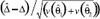 . The method for computing the degrees of freedom of the difference of normally-distributed simple random sample estimators with unequal variances from independent surveys is taken from Bickel and Doksum (1977). Section 6.4C recommends the Welch approximation, which computes as the degrees of freedom k for the estimating equation
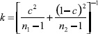 where
where
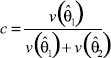 .
.
In our application n1 and n2 are both 50. If v(1) and v(2) are also both equal, then c = 1/2 and
![k equals the inverse of [the summation of {one-half squared divided by 49} and {one-half squared divided by 49}] which equals 98](/_images/scientific_equations-11.jpg)
That is the maximum value of k. If v(1) is much smaller, or much larger, than v(2), then
 .
.
49 is the minimum value of k. Thus 49 is the ‘conservative’ approximation for the degrees of freedom: it gives the widest confidence intervals (using the t distribution on 49 degrees of freedom). If v(1) and v(2) are unequal and both in the same order of magnitude, then Welch's approximation value can be used to generate an appropriate k, which will be in the range [49,98].
16The pseudo-values may not necessarily have a normal distribution: it is good practice to check this assumption and make sure there is not kurtosis which may reduce the effective degrees of freedom.
17It actually may be smaller if for a particular statistic many of the replicates are effectively equal to the full-sample estimator. 49 is actually the maximum in general.
Back to top
CANCER INFORMATION AND RESOURCES
PATIENT-ORIENTED INFORMATION
NCI's Cancer Information Service (CIS)
http://cis.nci.nih.gov/ with links to NCI-published fact sheets and other resources
Phone: 1-800-4-CANCER (1-800-422-6237)
TDD: 1-800-332-8615
Other NCI or DHHS Sources of Cancer Information
National Cancer Institute: www.cancer.gov
Office of Education and Special Initiatives (OESI): www.cancer.gov/aboutnci/oesi
Office of Communications: www.cancer.gov/aboutnci/office-of-communications/page3
American Cancer Society (ACS)
www.cancer.org/docroot/home/index.asp
FEDERALLY-SPONSORED PROGRAM PLANNING RESOURCES
Cancer Control P.L.A.N.E.T.
http://cancercontrolplanet.cancer.gov/
Research-tested Intervention Programs (RTIPs)
http://rtips.cancer.gov/rtips/index.do
Guide to Community Preventive Services
www.thecommunityguide.org/
RESEARCH TOOLS AND RESOURCES
Behavioral Risk Factor Surveillance System (BRFSS)
www.cdc.gov/brfss/
National Health Interview Survey (NHIS)
www.cdc.gov/nchs/nhis.htm
Current Population Survey (CPS)
www.census.gov/cps/
Surveillance, Epidemiology, and End Results (SEER)
http://seer.cancer.gov/
Pew Internet and American Life Project
http://www.pewinternet.org/data.asp
Back to top
Health Information Natitonal Survey (HINTS)
hints.cancer.gov
U.S. Department of Health and Human Services (DHHS)
National Institutes of Health (NIH)
National Cancer Institute (NCI)
NIH Publication No. 08-6435
Printed June 2008